Mesh functions¶

Included in the Python version of CALFEM is a mesh generation library based on GMSH. The library encapsulates the usage of GMSH transparently for the user. It will also parse the output from GMSH and create the necessary data structures required by CALFEM for solving finite element problems.

To use this functions in Python the mesh modules needs to be imported, which can be done with the following statements:

import calfem.geometry as cfg
import calfem.mesh as cfm

To visualise geometry and meshes we also optionally need the visualisation functions:

import calfem.vis_mpl as cfv

Mesh generation in CALFEM is divided in three steps:

1. Defining the geometry of the model.

2. Creating a finite element mesh with the desired elements and properties

3. Extracting data structures that can be used by CALFEM.

The following sections describe these steps.

Defining geometry¶

Geometry in CALFEM is described using the Geometry class. A Geometry-object will hold all points, lines and surfaces describing the geometry. This object is also what is passed to the mesh generation routines in the following sections.

A Geometry-object, g, is created with the following code:

g = cfg.Geometry()

This creates a Geometry object which will be used to described our geometry. Next we define the points that will be used to define lines, splines or ellipses. In this example we define a simple triangle:

g.point([0.0, 0.0]) # point 0
g.point([5.0, 0.0]) # point 1
g.point([2.5, 4.0]) # point 2

The points are connected together with spline-elements. These can have 2 or three nodes. In this case we only use 2 node splines (lines):

g.spline([0, 1]) # line 0
g.spline([1, 2]) # line 1
g.spline([2, 0]) # line 2

Finally we create the surface by defining what lines make up the surface:

g.surface([0, 1, 2])

To display our geometry, we use the calfem.vis module:

cfv.drawGeometry(g)
cfv.showAndWait()

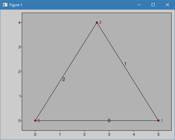
Running this example will show the following window with a simple triangle:

Creating a mesh¶

To create a mesh we need to create a GmshMesh object and initialize this with our geometry:

mesh = cfm.GmshMesh(g)

Next, we need to set some desired properties on our mesh:

mesh.el_type = 3          # Element type is quadrangle
mesh.dofs_per_node = 1     # Degrees of freedom per node
mesh.el_size_factor = 0.15 # Element size Factor

The el_type property determines the element used for mesh generation. Elements that can be generated are:

• 2 - 3 node triangle element

• 3 - 4 node quadrangle element

• 5 - 8 node hexahedron

• 16 - 8 node second order quadrangle

The dofs_per_node defines the number of degrees of freedom for each node. el_size_factor determines the coarseness of the mesh.

To generate the mesh and at the same time get the needed data structures for use with CALFEM we call the .create() method of the mesh object:

coords, edof, dofs, bdofs, elementmarkers = mesh.create()

The returned data structures are:

• coords - Element coordinates

• edof - Element topology

• dofs - Degrees of freedom per node

• bdofs - Boundary degrees of freedom. Dictionary containing the dofs for each boundary marker. More on markers in the next section.

• elementmarkers - List of integer markers. Row i contains the marker of element i. Can be used to determine what region an element is in.

To display the generated mesh we can use the drawMesh() function of the calfem.vis module:

cfv.figure()

# Draw the mesh.

cfv.drawMesh(
    coords=coords,
    edof=edof,
    dofs_per_node=mesh.dofsPerNode,
    el_type=mesh.elType,
    filled=True,
    title="Example 01"
)

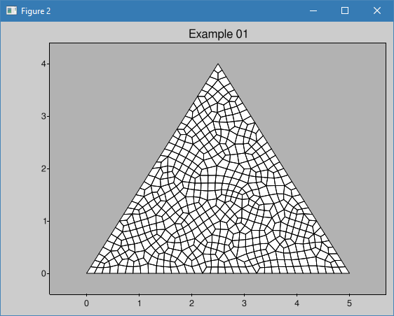
Running the example will produce the following mesh with quad elements:

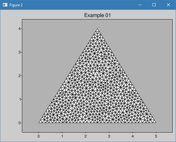
Changing the elType property to 2 (mesh.elType = 2) will produce a mesh with triangle elements instead:

Specifying boundary markers¶

To assist in assigning boundary conditions, markers can be defined on the geometry, which can be used to identify which dofs are assigned to nodes, lines and surfaces.

In this example we add a marker, 10, to line number 2. Markers are added as a parameter to the .spline() method of the Geometry object as shown in the following code:

g.spline([0, 1]) # line 0
g.spline([1, 2]) # line 1
g.spline([2, 0], marker=10) # line 2 with marker 10

It is also possible to assign markers to points. The marker parameter is added to the .point() method of the Geometry object.

g.point([0.0, 0.0])             # point 0
g.point([5.0, 0.0], marker=20)  # point 1
g.point([2.5, 4.0])             # point 2

In the same way markers can be added to surfaces as well.

Extracting dofs defined by markers¶

To extract the dofs defined by the marker we use the bdofs dictionary returned when the mesh was created by the .create() method. If we print the bdofs dictionary we get the following output:

{20: [2], 0: [1, 2, ... , 67], 10: [1, 3, 68, ... , 98]}

If we examine the output we see that there is a key, 10, containing the dofs of the number 2 line. We also have the key 20 with a single dof 2 in this case. If the dofsPerNode property in the mesh generator was set to 2 the marker 20 would have contained 2 integers.

For a more complete example see the XXX example.

Function reference¶

The following pages summarize selected mesh-related CALFEM functions.

calfem.geometry¶

calfem.geometry.geometry¶

Purpose:

No purpose text is available in the source docstring.

Syntax:

cfg.geometry()

Description:

Source docstring:

No description text is available in the source docstring.

calfem.mesh¶

calfem.mesh.create_mesh¶

Purpose:

Create a mesh for the given geometry using GMSH. This function serves as a convenient wrapper around the GmshMeshGenerator class to generate finite element meshes from geometric definitions.

Syntax:

cfm.create_mesh(geometry, el_type=2, el_size_factor=1, dofs_per_node=1, gmsh_exec_path=None, clcurv=False, min_size=None, max_size=None, meshing_algorithm=None, additional_options='')

Description:

Source docstring:

Create a mesh for the given geometry using GMSH.
This function serves as a convenient wrapper around the GmshMeshGenerator class
to generate finite element meshes from geometric definitions.
Parameters
----------
geometry : object
    The geometry object defining the domain to be meshed.
el_type : int, optional
    Element type identifier. Default is 2.
el_size_factor : float, optional
    Factor controlling the element size. Default is 1.
dofs_per_node : int, optional
    Number of degrees of freedom per node. Default is 1.
gmsh_exec_path : str, optional
    Path to the GMSH executable. If None, uses system default. Default is None.
clcurv : bool, optional
    Enable/disable curved element generation. Default is False.
min_size : float, optional
    Minimum element size constraint. Default is None.
max_size : float, optional
    Maximum element size constraint. Default is None.
meshing_algorithm : int, optional
    GMSH meshing algorithm identifier. Default is None.
additional_options : str, optional
    Additional GMSH options as a string. Default is ''.
Returns
-------
mesh : object
    The generated mesh object containing nodes, elements, and connectivity information.
Examples
--------
>>> mesh = create_mesh(geometry, el_type=3, el_size_factor=0.5)
>>> mesh = create_mesh(geometry, min_size=0.1, max_size=1.0)

calfem.mesh.trimesh2d¶

Purpose:

Triangulates an area described by a number vertices (vertices) and a set of segments that describes a closed polygon.

Syntax:

cfm.trimesh2d(vertices, segments=None, holes=None, maxArea=None, quality=True, dofs_per_node=1, logFilename='tri.log', triangleExecutablePath=None)

Description:

Source docstring:

Triangulates an area described by a number vertices (vertices) and a set
of segments that describes a closed polygon.

Parameters:

    vertices            array [nVertices x 2] with vertices describing the geometry.

                        [[v0_x, v0_y],
                         [   ...    ],
                         [vn_x, vn_y]]

    segments            array [nSegments x 3] with segments describing the geometry.

                        [[s0_v0, s0_v1,marker],
                         [        ...        ],
                         [sn_v0, sn_v1,marker]]

    holes               [Not currently used]

    maxArea             Maximum area for triangle. (None)

    quality             If true, triangles are prevented having angles < 30 degrees. (True)

    dofs_per_node         Number of degrees of freedom per node.

    logFilename         Filename for triangle output ("tri.log")

Returns:

    coords              Node coordinates

                        [[n0_x, n0_y],
                         [   ...    ],
                         [nn_x, nn_y]]

    edof                Element topology

                        [[el0_dof1, ..., el0_dofn],
                         [          ...          ],
                         [eln_dof1, ..., eln_dofn]]

    dofs                Node dofs

                        [[n0_dof1, ..., n0_dofn],
                         [         ...         ],
                         [nn_dof1, ..., nn_dofn]]

    bdofs               Boundary dofs. Dictionary containing lists of dofs for
                        each boundary marker. Dictionary key = marker id.

calfem.utils¶

calfem.utils.apply_bc¶

Purpose:

Apply boundary condition to bcPresc and bcVal matrices. For 2D problems with 2 dofs per node.

Syntax:

cfu.apply_bc(boundaryDofs, bcPrescr, bcVal, marker, value=0.0, dimension=0)

Description:

Source docstring:

Apply boundary condition to bcPresc and bcVal matrices. For 2D problems
with 2 dofs per node.

Parameters
----------
boundaryDofs : dict
    Dictionary with boundary dofs.
bcPresc : array_like
    1-dim integer array containing prescribed dofs.
bcVal : array_like
    1-dim float array containing prescribed values.
marker : int
    Boundary marker to assign boundary condition.
value : float, optional
    Value to assign boundary condition.
    If not given 0.0 is assigned.
dimension : int, optional
    dimension to apply bc. 0 - all, 1 - x, 2 - y

Returns
-------
bcPresc : array_like
    Updated 1-dim integer array containing prescribed dofs.
bcVal : array_like
    Updated 1-dim float array containing prescribed values.

calfem.utils.apply_bc_3d¶

Purpose:

Apply boundary condition to bcPresc and bcVal matrices. For 3D problems with 3 dofs per node.

Syntax:

cfu.apply_bc_3d(boundaryDofs, bcPrescr, bcVal, marker, value=0.0, dimension=0)

Description:

Source docstring:

Apply boundary condition to bcPresc and bcVal matrices. For 3D problems
with 3 dofs per node.

Parameters
----------
boundaryDofs : dict
    Dictionary with boundary dofs.
bcPrescr : array_like
    1-dim integer array containing prescribed dofs.
bcVal : array_like
    1-dim float array containing prescribed values.
marker : int
    Boundary marker to assign boundary condition.
value : float, optional
    Value to assign boundary condition.
    If not given 0.0 is assigned.
dimension : int, optional
    dimension to apply bc. 0 - all, 1 - x, 2 - y,
    3 - z

Returns
-------
bcPrescr : array_like
    Updated 1-dim integer array containing prescribed dofs.
bcVal : array_like
    Updated 1-dim float array containing prescribed values.

calfem.utils.apply_bc_node¶

Purpose:

Apply boundary conditions to a specific node. This function adds boundary condition prescriptions and values for a given node to existing boundary condition arrays.

Syntax:

cfu.apply_bc_node(nodeIdx, dofs, bcPrescr, bcVal, value=0.0, dimension=0)

Description:

Source docstring:

Apply boundary conditions to a specific node.
This function adds boundary condition prescriptions and values for a given node
to existing boundary condition arrays.

Parameters
----------
nodeIdx : int
    Index of the node to apply boundary conditions to.
dofs : array_like
    Degrees of freedom array. Can be 1D (for single DOF per node) or 2D
    (for multiple DOFs per node).
bcPrescr : array_like
    Existing array of prescribed boundary condition DOF indices.
bcVal : array_like
    Existing array of prescribed boundary condition values.
value : float, optional
    Value to prescribe for the boundary condition. Default is 0.0.
dimension : int, optional
    Dimension/direction to apply BC. If 0, applies to all DOFs of the node.
    If 1, 2, or 3, applies to specific dimension (1-indexed). Default is 0.

Returns
-------
tuple of numpy.ndarray
    A tuple containing:
    - Updated prescribed DOF indices array (bcPrescr concatenated with new DOFs)
    - Updated prescribed values array (bcVal concatenated with new values)

Notes
-----
When dimension=0, boundary conditions are applied to all degrees of freedom
for the specified node. When dimension is 1, 2, or 3, the boundary condition
is applied only to that specific dimension (using 1-based indexing).

Examples
--------
>>> # Apply BC to all DOFs of node 5 with value 0.0
>>> bc_dofs, bc_vals = apply_bc_node(5, dofs, [], [], 0.0, 0)
>>>
>>> # Apply BC to x-direction (dimension 1) of node 10 with value 5.0
>>> bc_dofs, bc_vals = apply_bc_node(10, dofs, bc_dofs, bc_vals, 5.0, 1)

calfem.utils.apply_force_node¶

Purpose:

Apply a force to a specific node in the finite element model. This function adds a force value to the global force vector at the degrees of freedom corresponding to a specified node. The force can be applied to all DOFs of the node or to a specific dimension.

Syntax:

cfu.apply_force_node(nodeIdx, dofs, f, value=0.0, dimension=0)

Description:

Source docstring:

Apply a force to a specific node in the finite element model.
This function adds a force value to the global force vector at the degrees of freedom
corresponding to a specified node. The force can be applied to all DOFs of the node
or to a specific dimension.
Parameters
----------
nodeIdx : int
    Index of the node where the force is to be applied.
dofs : array_like
    Degrees of freedom array that maps nodes to their DOF indices in the global system.
    Can be 1D (for single DOF per node) or 2D (for multiple DOFs per node).
f : array_like
    Global force vector where the force will be added.
value : float, optional
    Magnitude of the force to be applied. Default is 0.0.
dimension : int, optional
    Specific dimension/DOF to apply the force to. If 0, applies to all DOFs of the node.
    If 1 or higher, applies to the specified dimension (1-indexed). Default is 0.
Notes
-----
- When dimension=0, the force is applied to all DOFs of the node (assumes 1D dofs array)
- When dimension>=1, the force is applied to the specific dimension of the node
  (assumes 2D dofs array with shape [node, dimension])
- The dimension parameter uses 1-based indexing (dimension=1 corresponds to first DOF)
Examples
--------
>>> # Apply force to all DOFs of node 5
>>> apply_force_node(5, dofs, f, value=100.0, dimension=0)
>>> # Apply force to x-direction (dimension 1) of node 3
>>> apply_force_node(3, dofs, f, value=50.0, dimension=1)

calfem.utils.apply_force¶

Purpose:

Apply boundary force to f matrix. The value is added to all boundaryDofs defined by marker. Applicable to 2D problems with 2 dofs per node.

Syntax:

cfu.apply_force(boundaryDofs, f, marker, value=0.0, dimension=0)

Description:

Source docstring:

Apply boundary force to f matrix. The value is
added to all boundaryDofs defined by marker. Applicable
to 2D problems with 2 dofs per node.

Parameters:

    boundaryDofs        Dictionary with boundary dofs.
    f                   force matrix.
    marker              Boundary marker to assign boundary condition.
    value               Value to assign boundary condition.
                        If not given 0.0 is assigned.
    dimension           dimension to apply force. 0 - all, 1 - x, 2 - y

calfem.utils.apply_traction_linear_element¶

Purpose:

Apply traction on part of boundary with marker.

Syntax:

cfu.apply_traction_linear_element(boundaryElements, coords, dofs, F, marker, q)

Description:

Source docstring:

Apply traction on part of boundary with marker.

q is added to all boundaryDofs defined by marker. Applicable
to 2D problems with 2 dofs per node. The function works with linear
line elements. (elm-type 1 in GMSH).

Parameters
----------
boundaryElements : dict
    Dictionary with boundary elements, the key is a marker and the values are lists of elements.
coords : array_like
    Coordinates matrix
dofs : array_like
    Dofs matrix
F : array_like
    force matrix.
marker : int
    Boundary marker to assign boundary condition.
q : array_like
    Value to assign boundary condition.
    shape = [qx qy] in global coordinates

calfem.utils.apply_force_3d¶

Purpose:

Apply boundary force to f matrix for 3D problems. The value is added to all boundaryDofs defined by marker. Applicable to 3D problems with 3 degrees of freedom per node.

Syntax:

cfu.apply_force_3d(boundaryDofs, f, marker, value=0.0, dimension=0)

Description:

Source docstring:

Apply boundary force to f matrix for 3D problems.
The value is added to all boundaryDofs defined by marker. Applicable
to 3D problems with 3 degrees of freedom per node.
Parameters
----------
boundaryDofs : dict
    Dictionary with boundary degrees of freedom.
f : numpy.ndarray
    Force matrix to be modified.
marker : int or str
    Boundary marker to identify which boundary condition to apply.
value : float, optional
    Value to add to the force matrix at specified boundary DOFs.
    Default is 0.0.
dimension : int, optional
    Dimension to apply force:
    * 0 - all dimensions (default)
    * 1 - x-direction only
    * 2 - y-direction only
    * 3 - z-direction only
Notes
-----
If the specified marker does not exist in boundaryDofs, an error message
is printed. If an invalid dimension is specified (not 0, 1, 2, or 3),
an error message is printed.
Examples
--------
>>> boundaryDofs = {1: [1, 2, 3, 4, 5, 6]}
>>> f = np.zeros(6)
>>> apply_force_3d(boundaryDofs, f, 1, value=100.0, dimension=1)
# Applies force of 100.0 in x-direction to DOFs 1, 4

calfem.utils.apply_force_total¶

Purpose:

Apply boundary force to f matrix. Total force, value, is distributed over all boundaryDofs defined by marker. Applicable to 2D problems with 2 dofs per node.

Syntax:

cfu.apply_force_total(boundaryDofs, f, marker, value=0.0, dimension=0)

Description:

Source docstring:

Apply boundary force to f matrix. Total force, value, is
distributed over all boundaryDofs defined by marker. Applicable
to 2D problems with 2 dofs per node.

Parameters
----------
boundaryDofs : dict
    Dictionary with boundary dofs.
f : array_like
    Force matrix.
marker : int
    Boundary marker to assign boundary condition.
value : float, optional
    Total force value to assign boundary condition.
    If not given 0.0 is assigned.
dimension : int, optional
    Dimension to apply force. 0 - all, 1 - x, 2 - y

calfem.utils.apply_force_total_3d¶

Purpose:

Apply boundary force to f matrix. Total force, value, is distributed over all boundaryDofs defined by marker. Applicable to 3D problems with 3 dofs per node.

Syntax:

cfu.apply_force_total_3d(boundaryDofs, f, marker, value=0.0, dimension=0)

Description:

Source docstring:

Apply boundary force to f matrix. Total force, value, is
distributed over all boundaryDofs defined by marker. Applicable
to 3D problems with 3 dofs per node.

Parameters
----------
boundaryDofs : dict
    Dictionary with boundary dofs.
f : array_like
    Force matrix.
marker : int
    Boundary marker to assign boundary condition.
value : float, optional
    Total force value to assign boundary condition.
    If not given 0.0 is assigned.
dimension : int, optional
    Dimension to apply force. 0 - all, 1 - x, 2 - y,
    3 - z

calfem.vis_mpl¶

calfem.vis_mpl.draw_mesh¶

Purpose:

Draws wire mesh of model in 2D or 3D. Returns the Mesh object that represents the mesh.

Syntax:

cfv.draw_mesh(coords, edof, dofs_per_node, el_type, title=None, color=(0, 0, 0), face_color=(0.8, 0.8, 0.8), node_color=(0, 0, 0), filled=False, show_nodes=False)

Description:

Source docstring:

Draws wire mesh of model in 2D or 3D. Returns the Mesh object that represents
the mesh.

Parameters
----------
coords : ndarray
    An N-by-2 or N-by-3 array. Row i contains the x,y,z coordinates of node i.
edof : ndarray
    An E-by-L array. Element topology. (E is the number of elements and L is the number of dofs per element)
dofs_per_nodes : int
    Integer. Dofs per node.
el_type : int
    Integer. Element Type. See Gmsh manual for details. Usually 2 for triangles or 3 for quadrangles.
axes : matplotlib.axes.Axes, optional
    Matplotlib Axes. The Axes where the model will be drawn. If unspecified the current Axes will be used, or a new Axes will be created if none exist.
axes_adjust : bool, optional
    Boolean. True if the view should be changed to show the whole model. Default True.
title : str, optional
    String. Changes title of the figure. Default "Mesh".
color : tuple or str, optional
    3-tuple or char. Color of the wire. Defaults to black (0,0,0). Can also be given as a character in 'rgbycmkw'.
face_color : tuple or str, optional
    3-tuple or char. Color of the faces. Defaults to white (1,1,1). Parameter filled must be True or faces will not be drawn at all.
filled : bool, optional
    Boolean. Faces will be drawn if True. Otherwise only the wire is drawn. Default False.

calfem.vis_mpl.draw_elements¶

Purpose:

Draws wire mesh of model in 2D or 3D. Returns the Mesh object that represents the mesh.

Syntax:

cfv.draw_elements(ex, ey, title='', color=(0, 0, 0), face_color=(0.8, 0.8, 0.8), node_color=(0, 0, 0), line_style='solid', filled=False, closed=True, show_nodes=False)

Description:

Source docstring:

Draws wire mesh of model in 2D or 3D. Returns the Mesh object that represents
the mesh.

Parameters
----------
ex : ndarray
    Element x-coordinates array.
ey : ndarray
    Element y-coordinates array.
title : str, optional
    Changes title of the figure. Default "".
color : tuple or str, optional
    Color of the wire. Defaults to black (0,0,0). Can also be given as a character in 'rgbycmkw'.
face_color : tuple or str, optional
    Color of the faces. Defaults to (0.8,0.8,0.8). Parameter filled must be True or faces will not be drawn at all.
node_color : tuple or str, optional
    Color of the nodes. Defaults to black (0,0,0).
line_style : str, optional
    Line style for drawing. Default "solid".
filled : bool, optional
    Faces will be drawn if True. Otherwise only the wire is drawn. Default False.
closed : bool, optional
    Whether elements should be drawn as closed polygons. Default True.
show_nodes : bool, optional
    Whether to show nodes as markers. Default False.

calfem.vis_mpl.draw_node_circles¶

Purpose:

Draws wire mesh of model in 2D or 3D. Returns the Mesh object that represents the mesh.

Syntax:

cfv.draw_node_circles(ex, ey, title='', color=(0, 0, 0), face_color=(0.8, 0.8, 0.8), filled=False, marker_type='o')

Description:

Source docstring:

Draws wire mesh of model in 2D or 3D. Returns the Mesh object that represents
the mesh.

Parameters
----------
ex : ndarray
    Element x-coordinates array.
ey : ndarray
    Element y-coordinates array.
title : str, optional
    Changes title of the figure. Default "".
color : tuple or str, optional
    Color of the wire. Defaults to black (0,0,0). Can also be given as a character in 'rgbycmkw'.
face_color : tuple or str, optional
    Color of the faces. Defaults to (0.8,0.8,0.8). Parameter filled must be True or faces will not be drawn at all.
filled : bool, optional
    Faces will be drawn if True. Otherwise only the wire is drawn. Default False.
marker_type : str, optional
    Marker type for drawing. Default "o".

calfem.vis_mpl.draw_element_values¶

Purpose:

Draws scalar element values in 2D or 3D.

Syntax:

cfv.draw_element_values(values, coords, edof, dofs_per_node, el_type, displacements=None, draw_elements=True, draw_undisplaced_mesh=False, magnfac=1.0, title=None, color=(0, 0, 0), node_color=(0, 0, 0))

Description:

Source docstring:

Draws scalar element values in 2D or 3D.

Parameters
----------
values : array_like
    An N-by-1 array or a list of scalars. The Scalar values of the elements. ev[i] should be the value of element i.
coords : array_like
    An N-by-2 or N-by-3 array. Row i contains the x,y,z coordinates of node i.
edof : array_like
    An E-by-L array. Element topology. (E is the number of elements and L is the number of dofs per element)
dofs_per_node : int
    Dofs per node.
el_type : int
    Element Type. See Gmsh manual for details. Usually 2 for triangles or 3 for quadrangles.
displacements : array_like, optional
    An N-by-2 or N-by-3 array. Row i contains the x,y,z displacements of node i.
draw_elements : bool, optional
    True if mesh wire should be drawn. Default True.
draw_undisplaced_mesh : bool, optional
    True if the wire of the undisplaced mesh should be drawn on top of the displaced mesh. Default False. Use only if displacements != None.
magnfac : float, optional
    Magnification factor. Displacements are multiplied by this value. Use this to make small displacements more visible.
title : str, optional
    Changes title of the figure. Default "Element Values".
color : tuple or str, optional
    Color of the wire.
node_color : tuple or str, optional
    Color of the nodes.

calfem.vis_mpl.draw_displacements¶

Purpose:

Draws scalar element values in 2D or 3D. Returns the world object elementsWobject that represents the mesh.

Syntax:

cfv.draw_displacements(a, coords, edof, dofs_per_node, el_type, draw_undisplaced_mesh=False, magnfac=-1.0, magscale=0.25, title=None, color=(0, 0, 0), node_color=(0, 0, 0))

Description:

Source docstring:

Draws scalar element values in 2D or 3D. Returns the world object
elementsWobject that represents the mesh.

Parameters
----------
ev : array_like
    An N-by-1 array or a list of scalars. The Scalar values of the elements. ev[i] should be the value of element i.
coords : array_like
    An N-by-2 or N-by-3 array. Row i contains the x,y,z coordinates of node i.
edof : array_like
    An E-by-L array. Element topology. (E is the number of elements and L is the number of dofs per element)
dofs_per_node : int
    Dofs per node.
el_type : int
    Element Type. See Gmsh manual for details. Usually 2 for triangles or 3 for quadrangles.
displacements : array_like
    An N-by-2 or N-by-3 array. Row i contains the x,y,z  displacements of node i.
axes : matplotlib.axes.Axes
    Matlotlib Axes. The Axes where the model will be drawn. If unspecified the current Axes will be used, or a new Axes will be created if none exist.
draw_undisplaced_mesh : bool
    True if the wire of the undisplaced mesh should be drawn on top of the displaced mesh. Default False. Use only if displacements != None.
magnfac : float
    Magnification factor. Displacements are multiplied by this value. Use this to make small displacements more visible.
title : str
    Changes title of the figure. Default "Element Values".

calfem.vis_mpl.draw_ordered_polys¶

Purpose:

Draw ordered polygons on the current matplotlib axes.

Syntax:

cfv.draw_ordered_polys(o_polys)

Description:

Source docstring:

Draw ordered polygons on the current matplotlib axes.

This function takes a collection of ordered polygons and renders them as patches
on the current matplotlib axes. Each polygon is drawn with an orange face color
and a line width of 1.

Parameters
----------
o_polys : array-like
    A collection of polygons where each polygon is represented as a numpy array
    with shape (n_vertices, 2) or (n_vertices, 3+). Only the first two columns
    (x, y coordinates) are used for drawing.

Notes
-----
- The function uses the current matplotlib axes (plt.gca())
- All polygons are drawn with orange face color and line width of 1
- Only the first two columns of each polygon array are used for coordinates
- The function requires matplotlib.pyplot, matplotlib.path, and matplotlib.patches
  to be imported as plt, mpp, and patches respectively

Examples
--------
>>> import numpy as np
>>> import matplotlib.pyplot as plt
>>> # Create a simple triangle
>>> triangle = np.array([[0, 0], [1, 0], [0.5, 1], [0, 0]])
>>> draw_ordered_polys([triangle])
>>> plt.show()

calfem.vis_mpl.draw_nodal_values_contourf¶

Purpose:

Draw filled contour plot of nodal values on a finite element mesh. This function creates a filled contour plot (tricontourf) to visualize scalar values at the nodes of a finite element mesh. The contours are interpolated over triangular elements derived from the mesh topology.

Syntax:

cfv.draw_nodal_values_contourf(values, coords, edof, levels=12, title=None, dofs_per_node=None, el_type=None, draw_elements=False)

Description:

Source docstring:

Draw filled contour plot of nodal values on a finite element mesh.
This function creates a filled contour plot (tricontourf) to visualize scalar values
at the nodes of a finite element mesh. The contours are interpolated over triangular
elements derived from the mesh topology.
Parameters
----------
values : array_like
    Nodal values to be plotted as contours. Should have one value per node.
coords : array_like
    Node coordinates array with shape (n_nodes, 2) where each row contains
    [x, y] coordinates of a node.
edof : array_like
    Element topology array defining the connectivity between elements and
    degrees of freedom/nodes.
levels : int, optional
    Number of contour levels to draw. Default is 12.
title : str, optional
    Title for the plot. If None, no title is set. Default is None.
dofs_per_node : int, optional
    Number of degrees of freedom per node. Required if draw_elements is True.
    Default is None.
el_type : str, optional
    Element type identifier. Required if draw_elements is True. Default is None.
draw_elements : bool, optional
    Whether to overlay the mesh elements on the contour plot. If True,
    dofs_per_node and el_type must be specified. Default is False.
Notes
-----
- The function uses matplotlib's tricontourf for creating filled contours
- Element topology is converted to triangular connectivity using topo_to_tri
- The plot aspect ratio is set to 'equal' for proper geometric representation
- If draw_elements is True but required parameters are missing, an info message is displayed
Examples
--------
>>> coords = np.array([[0, 0], [1, 0], [0.5, 1]])
>>> edof = np.array([[1, 2, 3]])
>>> values = np.array([1.0, 2.0, 1.5])
>>> draw_nodal_values_contourf(values, coords, edof, levels=10, title="Temperature")

calfem.vis_mpl.draw_nodal_values_contour¶

Purpose:

Draw contour plot of nodal values on a triangulated mesh.

Syntax:

cfv.draw_nodal_values_contour(values, coords, edof, levels=12, title=None, dofs_per_node=None, el_type=None, draw_elements=False)

Description:

Source docstring:

Draw contour plot of nodal values on a triangulated mesh.

Parameters
----------
values : array_like
    Nodal values to be plotted as contours.
coords : array_like
    Coordinates of nodes in the mesh, shape (n_nodes, 2).
edof : array_like
    Element degrees of freedom connectivity matrix.
levels : int, optional
    Number of contour levels to draw, default is 12.
title : str, optional
    Title for the plot, default is None.
dofs_per_node : int, optional
    Number of degrees of freedom per node, required if draw_elements is True.
el_type : str, optional
    Element type, required if draw_elements is True.
draw_elements : bool, optional
    Whether to draw the mesh elements on top of contours, default is False.

Notes
-----
The function creates a triangulated contour plot using matplotlib's tricontour.
If draw_elements is True, both dofs_per_node and el_type must be specified
to draw the mesh overlay.

The plot uses equal aspect ratio and displays contours of the provided
nodal values interpolated over the triangulated mesh.

calfem.vis_mpl.draw_nodal_values_shaded¶

Purpose:

Draw shaded contour plot of nodal values using triangular interpolation. This function creates a shaded contour plot where nodal values are interpolated across triangular elements using Gouraud shading. The visualization shows smooth color gradients representing the variation of values across the mesh.

Syntax:

cfv.draw_nodal_values_shaded(values, coords, edof, title=None, dofs_per_node=None, el_type=None, draw_elements=False)

Description:

Source docstring:

Draw shaded contour plot of nodal values using triangular interpolation.
This function creates a shaded contour plot where nodal values are interpolated
across triangular elements using Gouraud shading. The visualization shows smooth
color gradients representing the variation of values across the mesh.
Parameters
----------
values : array-like
    Nodal values to be plotted. Should have one value per node.
coords : array-like
    Node coordinates as a 2D array with shape (n_nodes, 2) where each row
    contains [x, y] coordinates.
edof : array-like
    Element degrees of freedom connectivity matrix. Each row defines the
    nodes that belong to an element.
title : str, optional
    Title for the plot. If None, no title is displayed.
dofs_per_node : int, optional
    Number of degrees of freedom per node. Required if draw_elements is True.
el_type : str, optional
    Element type identifier. Required if draw_elements is True.
draw_elements : bool, default False
    If True, overlays the mesh elements on the contour plot. Requires
    dofs_per_node and el_type to be specified.
Notes
-----
- The function uses matplotlib's tripcolor with Gouraud shading for smooth
  interpolation between nodal values
- Element topology is converted to triangular format using topo_to_tri()
- If draw_elements is True but dofs_per_node or el_type are not provided,
  an informational message is displayed and the mesh is not drawn
- The plot aspect ratio is automatically set to equal for proper visualization
Examples
--------
>>> coords = np.array([[0, 0], [1, 0], [1, 1], [0, 1]])
>>> edof = np.array([[1, 2, 3], [1, 3, 4]])
>>> values = np.array([0.0, 1.0, 1.5, 0.5])
>>> draw_nodal_values_shaded(values, coords, edof, title="Temperature Distribution")

calfem.vis_mpl.draw_geometry¶

Purpose:

Draws the geometry (points and curves) in geoData.

Syntax:

cfv.draw_geometry(geometry, draw_points=True, label_points=True, label_curves=True, title=None, font_size=11, N=20, rel_margin=0.05, draw_axis=False, axes=None)

Description:

Source docstring:

Draws the geometry (points and curves) in geoData.

Parameters
----------
geometry : object
    GeoData object. Geodata contains geometric information of the model.
draw_points : bool, optional
    If True points will be drawn. Default True.
label_points : bool, optional
    If True Points will be labeled. The format is: ID[marker]. If a point has marker==0 only the ID is written. Default True.
label_curves : bool, optional
    If True Curves will be labeled. The format is: ID(elementsOnCurve)[marker]. Default True.
title : str, optional
    Title for the plot. Default None.
font_size : int, optional
    Size of the text in the text labels. Default 11.
N : int, optional
    The number of discrete points per curve segment. Default 20. Increase for smoother curves. Decrease for better performance.
rel_margin : float, optional
    Extra spacing between geometry and axis. Default 0.05.
draw_axis : bool, optional
    Whether to draw the axis frame. Default False.
axes : matplotlib.axes.Axes, optional
    Matplotlib Axes. The Axes where the model will be drawn. If unspecified the current Axes will be used, or a new Axes will be created if none exist. Default None.